
SE Inspect — a neuromorphic inspection cell you can build, read and reproduce
Two cameras, a Raspberry Pi 5, four BrainChip AKD1500 cards, a conveyor and a robot arm. Learns a part from ten photos in seconds, tells you which photo made the decision, and keeps running when a card dies. Non-commercial release planned.
Release status: The public source repository and installer are planned. The instructions described below are a preview; there is no public download yet.
In one minute
A part arrives on the belt. The Pi separates it from the belt — not trivially: the camera darkens towards the edges, the belt has texture, the lamps leave reflections. The silhouette goes to the AKD1500 cards, which learned this part from ten photos a minute ago, in about two milliseconds each. The verdict is GOOD, with the learned photo that won shown next to the live crop. The belt carries the part to the pickup zone; the arm takes it. If the part is unknown, the belt stops and the arm is never called. If a card hangs, the other three carry on and an alarm is written.
Everything on this page is either measured on that machine (with date, build and firmware), reproduced on a synthetic bench (with the script that draws the figure), or marked as open. A source-available, non-commercial release is planned; no public download exists yet.
Why this exists
The project began in August 2026 with no programming background, one AKD1500 and a question the product pages did not answer: what does neuromorphic hardware feel like when you make it do real work? The first evening was PCIe enumeration; the fifth day produced the principle the whole system still runs on — the Pi knows where, Akida knows what. The chronicle of those days is in the Lab Notes; this page is what they turned into.
Two things were decided early and never reversed. First, write down what failed: kernel patches, a card that hung, a numpy version that killed the camera, five photos of empty belt that turned a class into an everything-matcher. Second, keep three kinds of statements apart: vendor facts, our measurements, our experiments. This page follows that rule; the labels are on every section.
The system
| Where | What | Why there |
|---|---|---|
| Raspberry Pi 5 | capture, belt model, segmentation, contours, geometry, tracking, fusion, line state, alarms, recipes, UI | spatial reasoning needs pixel coordinates and is cheap on a CPU |
| AKD1500 cards 0–2 | the silhouette ensemble: each card holds a third of the learned views; best match wins | prototype learning on the chip — learning in milliseconds, no gradients, and the winning neuron points back to a photo |
| AKD1500 card 3 | SE-M3, the one-pass detector for several, overlapping parts | the research goal: one card, one hardware sequence, one pass |
| Belt, relay, arm | 12 V motor behind a relay on GPIO 18; RAMPS/Arduino stepper arm on USB | the physical consequence of a wrong verdict — the reason the verdict has to be honest |
One process on the Pi runs all of it (tools/run_web.py, as a systemd service); the UI is a single HTML file talking to ~60 JSON endpoints. No cloud, no GPU, no framework on the runtime side beyond OpenCV and the Akida runtime.
What makes it different
1. It learns at the machine, in seconds. Ten photos, one click, "Step 3 of 3 · 0.3 s". The cards store prototypes; there is no training run to wait for and no model file to ship. (OUR OBSERVATION, 2026-09-20, build 1.9.36: 79 examples, 3 objects.)
2. It tells you why. After learning, every photo is replayed and attached to the neuron that fires strongest for it. At runtime the verdict shows the live crop next to that photo — "Neuron 3 · Card 2". A wrong verdict is a wrong photo you can delete. No saliency maps, no second model.
3. It refuses to guess. A confidence threshold turns a weak match into unknown instead of the best wrong name; the unknown rate is a first-class number with a retrain trigger; an unknown part at pickup stops the belt and never calls the arm; a photo without a freeable part is not learned.
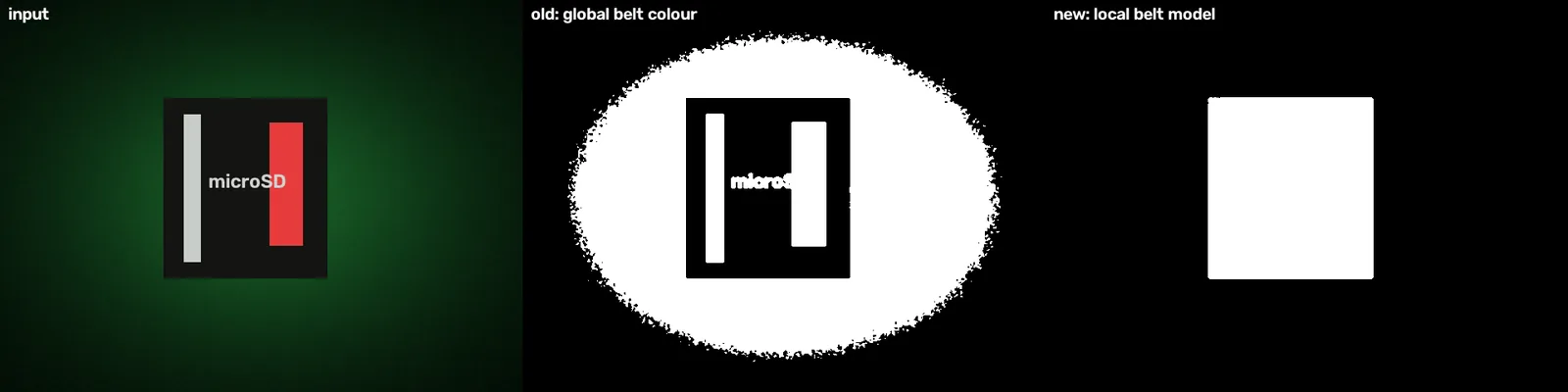
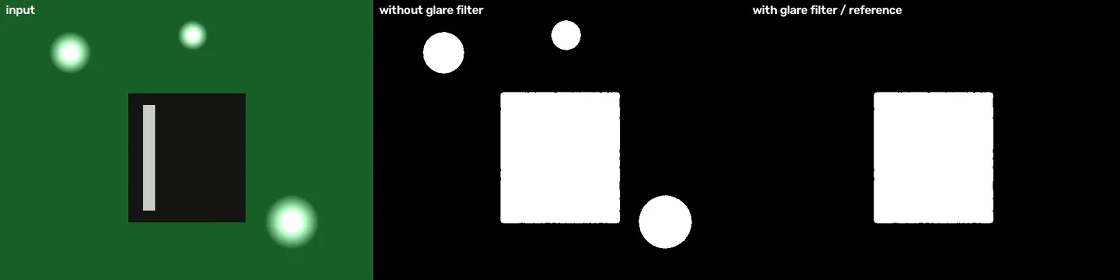
4. The hard part happened before the network — and it is documented. Vignetting made the labels easier than the card; lamp reflections became parts; a single empty-belt image could not know the flicker. The fixes — a local belt model, a 16-frame reference with a per-pixel noise map, a glare filter, a hole signature that splits a "carabiner around an SD card" — each come with a bench script that draws its own before/after figure.
5. It keeps running. Since build 1.9.36 every card shows its current task, last compute time and calls per second. A card that throws leaves the ensemble, the others answer, an alarm is written, a rejoin is tried after 60 s, and a button performs the PCIe reset that we first did by hand on 20 September. (The incident and its dmesg lines are in Demo 00.)
6. It is a line, not a demo. A state machine with two modes — flow (the belt runs, stops briefly to inspect each part, stops for the arm) and single — with timeouts, a störung state, an inspection log with CSV export, an ISA-101-style alarm book and recipes per part variant.
The vision pipeline, honestly
What a frame goes through, in order, and what each step cost us to learn:
- Belt model. Not one background colour but a smooth 4th-order surface per Lab channel, fitted robustly over five rounds of shrinking tolerance so parts drop out as outliers. Why: a single colour from the frame border sits ~31 units from the bright centre of a vignetted image; a black card falls below that, its white label does not. (BENCH: IoU 0.98 vs 0.07.)
- Edge silhouette. Anything enclosed by closed colour edges and unreachable from the border is a part, whatever is printed inside it.
- Empty-belt reference. 16 frames over ~2 s: median = reference, largest per-pixel deviation = noise map, threshold per pixel. Recorded with the belt running, the map contains the belt texture in every phase.
- Glare filter. Saturated spots in small blobs plus a halo of 1.8 × their radius are never parts; large white parts are untouched.
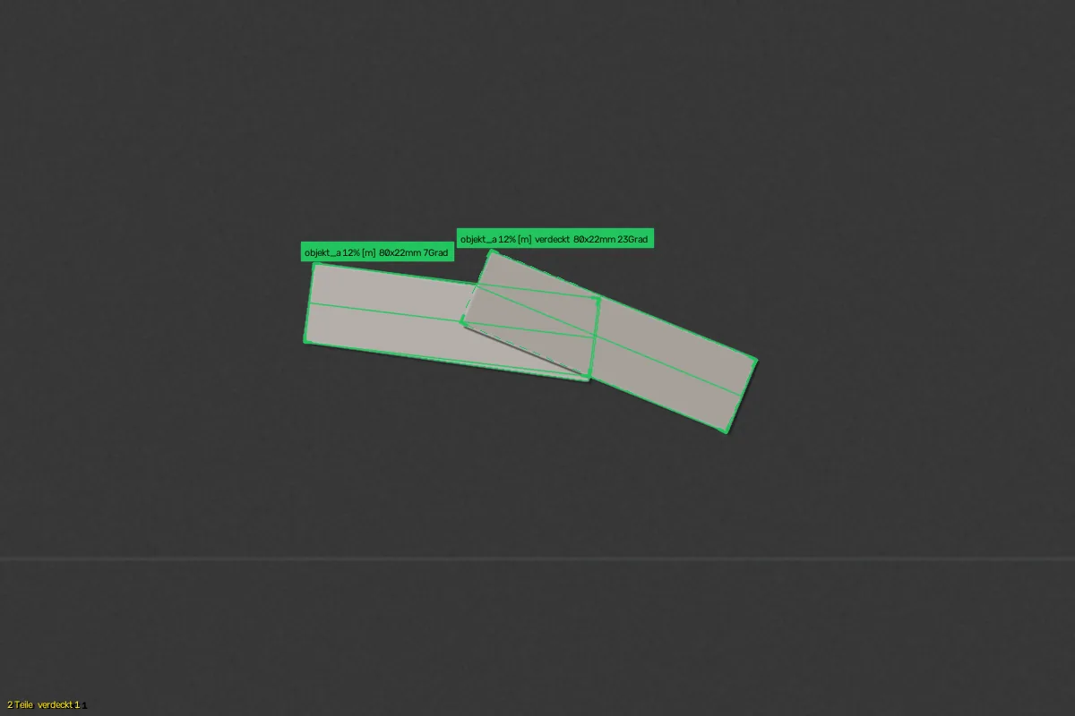
- Watershed and rectangle decomposition for touching and overlapping parts; a hole signature learned per class vetoes physically impossible verdicts and splits the blob along the hole.
- Silhouette → cards. 48 × 48, two channels, binary. Best match over the ensemble; confidence = share of the stored pattern found again.
- Fusion with the M3 detector's candidates when present ("find and confirm"), and with a second camera on the delivery zone: agreement → stronger + 0.08; disagreement → a view wins only at ≥ 0.80 against < 0.55, else unknown.
The line
Flow mode, the default since build 1.9.33: the belt runs by itself; a part entering the delivery zone stops it for a stable verdict (or "unknown" after 4 s); the belt continues; every further part stops it again; a known part at pickup stops it for the arm, and the camera — not the arm — decides when the cycle is done (zone empty for 0.6 s). The verdict is booked in the delivery zone, so the inspection log counts parts, not pickups.
The bench runs a whole shift in one second: lauf> → pruefen| → lauf> → pruefen| → lauf> → zone| → arm| → lauf> → … → stoerung| → lauf> → aus| (Demo 07). The timing constants are bench values; tuning on the real belt is an open point.
The operator interface
UI 2.2 follows high-performance-HMI ideas (ISA-101): grey surfaces, colour only for state, seven navigation entries in three groups, an operator view that hides everything an operator does not need and an expert view that shows it. One camera-control strip — the same under the main image and on every zone tile. Settings live where their effect is visible: camera under the image, threshold under the verdict, overlays in an eye menu. The old seven-tab settings dialog is gone; a "Status" area bundles hardware (with the live task per card and the reset button), diagnostics and maintenance.
SE-M3 — the detector
(EXPERIMENTAL.) A compact detector for the AKD1500: each grid cell emits three equal object slots — up to three overlapping parts per position — plus an overflow signal that says "more than I can describe here" instead of inventing a count. Anchor-free; angles as sin 2θ / cos 2θ; slots have no fixed order, so training matches predictions to targets over all permutations (M! ≤ 24); post-processing never suppresses two slots of the same cell against each other.
Variant V6 (256 px, 32 × 32 grid, 8-px cells) maps to one sequence, one pass, 18 of 32 NPs (OUR OBSERVATION, 2026-08-26, firmware BC.A1.003.009, MetaTF 2.19.3) — checked before training, with two deliberately invalid variants that must fail. What is open: detection quality on real images. We say so on every page that mentions M3.
Documented state
| Value | Kind | Where | |
|---|---|---|---|
| Learning time per example | ~2 ms | measured | Evidence → Measurements |
| Chip learning, 79 examples / 3 objects | < 1 s (step 3/3: 0.3 s) | measured, 2026-09-20 | Demo 03 |
| V6 mapping | 1 sequence · 1 pass · 18/32 NPs | measured, 2026-08-26 | Demo 02 |
| Camera → verdict | 22.7 ms (one frame, touching-parts scene, Aug 2026, incl. segmentation) | measured, build 1.2.6 | Evidence → Methods |
| Belt model on vignetting | card IoU 0.98 (was 0.07) | bench | Demo 05 |
| Reference pipeline | 0.22 mm / 0.33° median | bench | Demo 08 |
| Card recovery | remove/rescan < 10 s, no reboot | measured, 2026-09-20 | Demo 00 |
Not claimed: AKD1500 power (no sensor exposed for this chip in MetaTF 2.19.3), energy per object, M3 accuracy. Full table with limits: Evidence → Measurements.
What we learned (the short list)
Two numpy worlds on one Pi. Map before you train — and make the test able to fail. Verify the build string on the machine. Make every rejection explain itself. Empty negatives poison a class. Vignetting beats global thresholds. One empty frame is not a background model. Angles must move with the image. Handed parts are not mirrorable. Image the SD card. Kernel updates are hardware events. One file, one editor. Fix glare at the lamp. (Each is a paragraph with date and cost in the Lab Note "Thirteen expensive lessons".)
Get it, run it, cite it
A source-available release under PolyForm Noncommercial 1.0.0 is planned for research, teaching and private benches; commercial arrangements would be handled separately. It is not open source in the OSI sense, and we say so. BrainChip's driver and SDK come from BrainChip under their terms; we link, we do not bundle.
The planned release will offer three ways in: five minutes without hardware (python3 tools/run_web.py --synthetisch), thirty minutes with one card (the guide, or the planned install.sh), or the full cell (twelve guide chapters, parts list included). Contributions are planned under DCO + CLA. Verified hardware, BibTeX and a release DOI will be published with the repository.
Read the guide →Explore the demosEvidenceGet SE Inspect
Roadmap
Next: the self-learning cell — collect unknown cases, propose new classes from clusters, retrain with one click in seconds. Then: one-class operation, an energy-per-object measurement with an external meter on the carrier's 5 V input, a YOLO-class comparison model on the same data, weight-bank paging, learned-state transfer between cells, OPC UA/MQTT, dimensional checks, and roles/PIN with an audit trail.
Credits and independence
Built by Andreas Thurmayr, Ruhpolding. Code implemented with Claude; design and documentation direction with ChatGPT; every claim verified on the bench or on a script in the repository. SpikingEdge is an independent developer project, not affiliated with, endorsed by or sponsored by BrainChip, Inc.